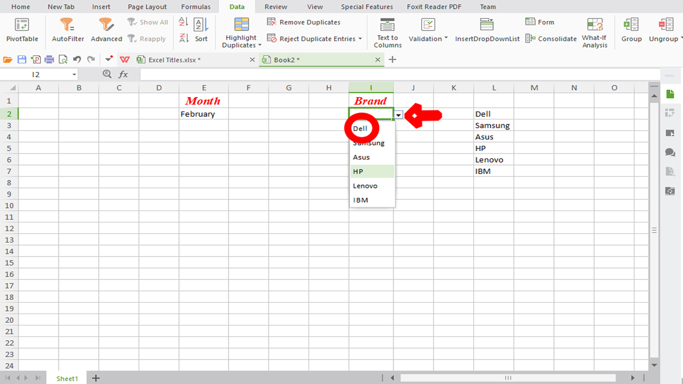
Excel is an important tool for data management and analysis, and the ability to create a drop-down list is a great feature for effective data entry. A drop-down list in Excel is a list of values that users can choose from when entering data into a cell. This feature helps to reduce data entry errors and ensures consistency in data entry. In this article, we will discuss how to create a drop-down list in Excel.
Step 1: Create a List of Items
Before creating a drop-down list, you need to create a list of items that will be displayed in the list. To create the list, follow these steps:
- Open a new or existing worksheet in Excel.
- Select the cells where you want to create the list.
- Type the list of items in the cells, with each item in a separate cell.
For example, if you want to create a list of countries, you can type the names of the countries in separate cells, as shown below:
Step 2: Create a Named Range
After creating the list of items, you need to create a named range that refers to the cells that contain the list. A named range is a group of cells that can be referred to by a name instead of a cell reference. To create a named range, follow these steps:
- Select the cells that contain the list of items.
- Click on the “Formulas” tab in the Excel ribbon.
- Click on the “Define Name” button in the “Defined Names” group.
- In the “New Name” dialog box, type a name for the range in the “Name” field.
- Click on the “OK” button to create the named range.
For example, if you want to create a named range for the list of countries, you can name it “CountriesList”, as shown below:
Step 3: Create the Drop-Down List
Now that you have created the list of items and a named range that refers to the cells that contain the list, you can create the drop-down list. To create the drop-down list, follow these steps:
- Select the cell where you want to create the drop-down list.
- Click on the “Data” tab in the Excel ribbon.
- Click on the “Data Validation” button in the “Data Tools” group.
- In the “Data Validation” dialog box, select “List” in the “Allow” field.
- In the “Source” field, type the name of the named range that you created in step 2.
- Click on the “OK” button to create the drop-down list.
Step 4: Test the Drop-Down List
To test the drop-down list, select the cell that contains the drop-down list and try selecting different items from the list. The cell will only accept values from the list, and if you try to type in a value that is not in the list, you will get an error message. The drop-down list feature is very useful when you have a lot of data to input. It ensures that the data is consistent, accurate, and saves time.
Some of the benefits of using a drop-down list in Excel include:
Ensures data accuracy: With a drop-down list, you can control the data entered into a cell. It ensures that users input data that is accurate and valid.
Saves time: The drop-down list feature saves time by providing users with a list of options to choose from. It eliminates the need for users to type in data, which can be time-consuming.
Reduces errors: The drop-down list feature reduces errors by limiting the options that users can choose from. It ensures that users do not enter incorrect data.
Increases consistency: The drop-down list feature increases consistency by ensuring that all the data entered is in the same format. It eliminates variations that can occur when users enter data manually.
Conclusion
creating a drop-down list in Excel is a simple process that can save time, increase accuracy, and improve data consistency. It is an essential feature for data entry, and it can be used in various applications such as budgeting, inventory management, and data analysis. By following the steps outlined above, you can create a drop-down list in Excel and improve your data management and analysis capabilities.
Zeeshan is a seasoned tech expert and senior writer at Teckrr.com. With over 10 years of experience in tech journalism, he brings insightful analysis and up-to-date information on the latest tech trends. Zeeshan holds a MBA degree from Business and Tech University and is known for his engaging writing style and ability to demystify complex tech topics. Stay connected with the cutting-edge of technology through his expert lens.

Leave a Reply